Visualizing GitHub’s global community

This is the second post in a series about how we built our new homepage.

1. How our globe is built
2. How we collect and use the data behind the globe
3. How we made the page fast and performant
4. How we illustrate at GitHub
5. How we designed the homepage and wrote the narrative

In the first post, my teammate Tobias shared how we made the 3D globe come to life, with lots of nitty gritty details about Three.js, performance optimization, and delightful touches.

But there’s another side to the story—the data! We hope you enjoy the read. ✨

Data goals

When we kicked off the project, we knew that we didn’t want to make just another animated globe. We wanted the data to be interesting and engaging. We wanted it to be real, and most importantly, we wanted it to be live.

Luckily, the data was there.

The challenge then became designing a data service that addressed the following challenges:

1. How do we query our massive volume of data?
2. How do we show you the most interesting bits?
3. How do we geocode user locations in a way that respects privacy?
4. How do we expose the computed data back to the monolith?
5. How do we not break GitHub? 😊

Let’s begin, shall we?

Querying GitHub

So, how hard could it be to show you some recent pull requests? It turns out it’s actually very simple:

class GlobeController < ApplicationController
  def data
    pull_requests = PullRequest
      .where(open: true)
      .joins(:repositories)
      .where("repository.is_open_source = true")
      .last(10_000)

    render json: pull_requests
  end
end

Just kidding 😛

Because of the volume of data generated on GitHub every day, the size of our databases, as well as the importance of keeping GitHub fast and reliable, we knew we couldn’t query our production databases directly.

Luckily, we have a data warehouse and a fantastic team that maintains it. Data from production is fetched, sanitized, and packaged nicely into the data warehouse on a regular schedule. The data can then be queried using Presto, a flavor of SQL meant for querying large sets of data.

We also wanted the data to be as fresh as possible. So instead of querying snapshots of our MySQL tables that are only copied over once a day, we were able to query data coming from our Apache Kafka event stream that makes it into the data warehouse much more regularly.

As an example, we have an event that is reported every time a pull request is merged. The event is defined in a format called protobuf, which stands for “protocol buffer.”

Here’s what the protobuf for a merged pull request event might look like:

message PullRequestMerge {
  github.v1.entities.User actor = 1;
  github.v1.entities.Repository repository = 2;
  github.v1.entities.User repository_owner = 3;
  github.v1.entities.PullRequest pull_request = 4;
  github.v1.entities.Issue issue = 5;
}

Each row corresponds to an “entity,” each of which is defined in its own protobuf file. Here’s a snippet from the definition of a pull request entity:

message PullRequest {
  uint64 id = 1;
  string global_relay_id = 2;
  uint64 author_id = 3;

  enum PullRequestState {
    UNKNOWN = 0;
    OPEN = 1;
    CLOSED = 2;
    MERGED = 3;
  }
  PullRequestState pull_request_state = 4;

  google.protobuf.Timestamp created_at = 5;
  google.protobuf.Timestamp updated_at = 6;
}

Including an entity in an event will pass along all of the attributes defined for it. All of that data gets copied into our data warehouse for every pull request that is merged.

This means that a Presto query for pull requests merged in the past day could look like:

SELECT
  pull_request.created_at,
  pull_request.updated_at,
  pull_request.id,
  issue.number,
  repository.id
FROM kafka.github.pull_request_merge
WHERE
  day >= CAST((CURRENT_DATE - INTERVAL '1' DAY) AS VARCHAR)

There are a few other queries we make to pull in all the data we need. But as you can see, this is pretty much standard SQL that pulls in merged pull requests from the last day in the event stream.

Surfacing interesting data

We wanted to make sure that whatever data we showed was interesting, engaging, and appropriate to be spotlighted on the GitHub homepage. If the data was good, visitors would be enticed to explore the vast ecosystem of open source being built on GitHub at that given moment. Maybe they’d even make a contribution!

So how do we find good data?

Luckily our data team came to the rescue yet again. A few years ago, the Data Science Team put together a model to rank the “health” of repositories based on 30-plus features weighted by importance. A healthy repository doesn’t necessarily mean having a lot of stars. It also takes into account how much current activity is happening and how easy it is to contribute to the project, to name a few.

The end result is a numerical health score that we can query against in the data warehouse.

SELECT repository_id
FROM data_science.github.repository_health_scores
WHERE 
  score > 0.75

Combining this query with the above, we can now pull in merged pull requests from repositories with health scores above a certain threshold:

WITH
healthy_repositories AS (
  SELECT repository_id
  FROM data_science.github.repository_health_scores
  WHERE 
    score > 0.75
)

SELECT
  a.pull_request.created_at,
  a.pull_request.updated_at,
  a.pull_request.id,
  a.issue.number,
  a.repository.id
FROM kafka.github.pull_request_merge a
JOIN healthy_repositories b
ON a.repository.id = b.repository_id
WHERE
  day >= CAST((CURRENT_DATE - INTERVAL '1' DAY) AS VARCHAR)

We do some other things to ensure the data is good, like filtering out accounts with spammy behavior. But repository health scores are definitely a key ingredient.

Geocoding user-provided locations

Your GitHub profile has an optional free text field for providing your location. Some people fill it out with their actual location (mine says “San Francisco”), while others use fake or funny locations (42 users have “Middle Earth” listed as theirs). Many others choose to not list a location. In fact, two-thirds of users don’t enter anything and that’s perfectly fine with us.

For users that do enter something, we try to map the text to a real location. This is a little harder to do than using IP addresses as proxies for locations, but it was important to us to only include data that users felt comfortable making public in the first place.

In order to map the free text locations to latitude and longitude pairs, we use Mapbox’s forward geocoding API and their Ruby SDK. Here’s an example of a forward geocoding of “New York City”:

MAPBOX_OPTIONS = {
  limit: 1,
  types: %w(region place country),
  language: "en"
}

Mapbox::Geocoder.geocode_forward("New York City", MAPBOX_OPTIONS)

=> [{
  "type" => "FeatureCollection",
  "query" => ["new", "york", "city"],
  "features" => [{
    "id" => "place.15278078705964500",
    "type" => "Feature",
    "place_type" => ["place"],
    "relevance" => 1,
    "properties" => {
      "wikidata" => "Q60"
    },
    "text_en" => "New York City",
    "language_en" => "en",
    "place_name_en" => "New York City, New York, United States",
    "text" => "New York City",
    "language" => "en",
    "place_name" => "New York City, New York, United States",
    "bbox" => [-74.2590879797556, 40.477399, -73.7008392055224, 40.917576401307],
    "center" => [-73.9808, 40.7648],
    "geometry" => {
      "type" => "Point", "coordinates" => [-73.9808, 40.7648]
    },
    "context" => [{
      "id" => "region.17349986251855570",
      "wikidata" => "Q1384",
      "short_code" => "US-NY",
      "text_en" => "New York",
      "language_en" => "en",
      "text" => "New York",
      "language" => "en"
    }, {
      "id" => "country.19678805456372290",
      "wikidata" => "Q30",
      "short_code" => "us",
      "text_en" => "United States",
      "language_en" => "en",
      "text" => "United States",
      "language" => "en"
    }]
  }],
  "attribution" => "NOTICE: (c) 2020 Mapbox and its suppliers. All rights reserved. Use of this data is subject to the Mapbox Terms of Service (https://www.mapbox.com/about/maps/). This response and the information it contains may not be retained. POI(s) provided by Foursquare."
}, {}]

There is a lot of data there, but let’s focus on text, relevance, and center for now. Here are those fields for the “New York City”:

result = Mapbox::Geocoder.geocode_forward("New York City", MAPBOX_OPTIONS)
result[0]["features"][0].slice("text", "relevance", "center")

=> {"text"=>"New York City", "relevance"=>1, "center"=>[-73.9808, 40.7648]}

If you use “NYC” query string, you get the exact same result:

result = Mapbox::Geocoder.geocode_forward("NYC", MAPBOX_OPTIONS)
result[0]["features"][0].slice("text", "relevance", "center")

=> {"text"=>"New York City", "relevance"=>1, "center"=>[-73.9808, 40.7648]}

Notice that the text is still “New York City” in this second example? That is because Mapbox is normalizing the results. We use the normalized text on the globe so viewers get a consistent experience. This also takes care of capitalization and misspellings.

The center field is an array containing the longitude and latitude of the location.

And finally, the relevance score is an indicator of Mapox’s confidence in the results. A relevance score of 1 is the highest, but sometimes users enter locations that Mapbox is less sure about:

result = Mapbox::Geocoder.geocode_forward("Middle Earth", MAPBOX_OPTIONS)
result[0]["features"][0].slice("text", "relevance", "center")

=> {"text"=>"Earth City", "relevance"=>0.5, "center"=>[-90.4682, 38.7689]}

We discard anything with a score of less than 1, just to get confidence that the location we show feels correct.

Mapbox also provides a batch geocoding endpoint. This allows us to query multiple locations in one request:

MAPBOX_ENDPOINT = "mapbox.places-permanent"

query_string = "{San Francisco};{Berlin};{Dakar};{Tokyo};{Lima}"

Mapbox::Geocoder.geocode_forward(query_string, MAPBOX_OPTIONS, MAPBOX_ENDPOINT)

After we’ve geocoded and normalized all of the results, we create a JSON representation of the pull request and its locations so our globe JavaScript client knows how to parse it.

Here’s a pull request we recently featured that was opened in San Francisco and merged in Tokyo:

{
   "uml":"Tokyo",
   "gm":{
      "lat":35.68,
      "lon":139.77
   },
   "uol":"San Francisco",
   "gop":{
      "lat":37.7648,
      "lon":-122.463
   },
   "l":"JavaScript",
   "nwo":"mdn/browser-compat-data",
   "pr":7937,
   "ma":"2020-12-17 04:00:48.000",
   "oa":"2020-12-16 10:02:31.000"
}

We use short keys to shave off some bytes from the JSON we end up serving so the globe loads faster.

Airflow, HDFS, and Munger

We run our data warehouse queries and geocoding throughout the day to ensure that the data on the homepage is always fresh.

For scheduling this work, we use another system from Apache called Airflow. Airflow lets you run scheduled jobs that contain a sequence of tasks. Airflow calls these workflows Direct Acyclical Graphs (or DAGs for short), which is a borrowed term from graph theory in computer science. Basically this means that you schedule one task at a time, execute the task, and when the task is done, then the next task is scheduled and eventually executed. Tasks can pass along information to each other.

At a high level, our DAG executes the following tasks:

1. Query the data warehouse.
2. Geocode locations from the results.
3. Write the results to a file.
4. Expose the results to the GitHub Rails app.

We covered the first two steps earlier. For writing the file, we use HDFS, which is a distributed file system that’s part of the Apache Hadoop project. The file is then uploaded to Munger, an internal service we use to expose results from the data science pipeline back to the GitHub Rails app that powers github.com.

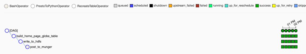
Here’s what this might look like in the Airflow UI:

Each column in that screenshot represents a full DAG run of all of the tasks. The last column with the light green circle at the top indicates that the DAG is in the middle of a run. It’s completed the build_home_page_globe_table task (represented by a dark green box) and now has the next task write_to_hdfs scheduled (dark blue box).

Our Airflow instance runs more than just this one DAG throughout the day, so we may stay in this state for some time before the scheduler is ready to pick up the write_to_hdfs task. Eventually the remaining tasks should run. If everything ends up running smoothly, we should see all green:

Wrapping up

Hope that gives you a glimpse into how we built this!

Again, thank you to all the teams that made the GitHub homepage and globe possible. This project would not have been possible without years of investment in our data infrastructure and data science capabilities, so a special shout out to Kim, Jeff, Preston, Ike, Scott, Jamison, Rowan, and Omoju.

More importantly, we could not have done it without you, the GitHub community, and your daily contributions and projects that truly bring the globe to life. Stay tuned—we have even more in store for this project coming soon.

In the meantime, I hope to see you on the homepage soon. 😉